Overview Data Preparation Topic Modeling Sentiment Analysis Outcome and Reflection
Sentiment Analysis
Introduction
Sentiment analysis is a text classification task, in which the goal is to analyze a text and discover opinions and classify the sentiment they convey to determine the writer’s attitude towards a specific object, aspect, brand, etc.
As described in the Overview section, our dataset contains open answers to an employee survey about what goes well and not so well at a company. Looking at the comments we could derive a set of criteria that was necessary for the approach we chose:
- scalability - while the current dataset only contained 17,672 comments, we want our approach to be able to handle much larger amounts of data as well
- transferability - we want to be able to perform sentiment analysis on various topics and types of text
- achieve best performance with minimal labeled data
Generally there are three types of approaches to sentiment analysis (SA): lexicon-based (or rule-based), non-neural-network classifiers, and neural-network classifiers. Our first criterion rules out the lexicons-based methods. While these have their advantages for very specific texts, they are not suitable on our large, irregular, and noisy data. For our purposes, a dynamic approach is needed, that can adapt to any type of dataset without significant modifications
Support Vector Machines (SVM) is one non-neural-network approach that we considered. However, from our previous experience with machine learning techniques, they achieve similar performance, but tend to not scale as well on larger datasets, and also require more feature engineering than Neural Networks.
Additionally we want our approach to handle, if needed, large amounts of irregular and noisy data which more traditional SA methods cannot do well. (Liu et. al, 2019) Moreover, neural network methods offer other benefits, such as adaptive learning, parallelism for increased computational efficiency and easier generalization over domains. (Chen et. al, 2011)
When it comes to neural-network approaches, there are many to choose from: for the task of SA the most popular ones are Recurrent Neural Networks (RNN) (Zhang et al, 2018), regular and hybrid Convolutional Neural Networks (CNN) (Wang et al, 2016), Transformers, as well as many combinations of the previously mentioned ones and lexicon-based techniques.
We had two specific goals in mind: one was to implement and fine-tune a NN ourselves, and the second one to use an out-of-the-box approach and see how they compare in performance. For these reasons we settled on two architectures: an LSTM which incorporates lexical features, and the BERT approach (Bidirectional Encoder Representations) as a way of experimenting with transfer learning.
It is worth mentioning that there are multiple BERT-like architectures that offer either less computational cost while retaining most of BERTs language understanding capabilities (e.g. DistilBERT (Sanh et. al, 2019), ALBERT (Lan et. al, 2019)), or improved performance for increases in computational demand (e.g. XLNet (Yang et. al 2019), RoBERTa (Liu et. al, 2019)). We selected the BERT architecture over the other options as it represents a middle ground between speed and accuracy.
Labeling the dataset
Most machine learning SA approaches are supervised, which means that a labeled dataset is needed in order to train the model. NN approaches need large amounts of data so often, they use datasets in which the labels are already contained and don’t have to be manually created. For instance, review corpora contain the user’s rating of a product, movie, service, etc., in addition to the review text. This way, the ratings can be used as labels, in order to predict what the user’s sentiment towards what they are reviewing.
Our dataset did not contain such meta-information, therefore an extra step was required in which we labeled a part of the comments ourselves. There are many ways to sentiment-label a dataset. Cambria (2016) divided this task into sentiment recognition (identifying a set of emotions tags in a text e.g. sadness, anger) and polarity detection (e.g. positive vs. negative, like vs. not like). We chose a three-point polarity labeling frame: positive, neutral, negative. The manual labeling was performed by three of the group members, who annotated 300 comments per each of the two questions, leading to a total of 600 labeled comments.
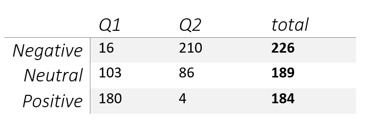
The comments proved to be highly ambiguous, making it difficult to decide whether a text was positive, negative or neutral. In the end the annotators chose the same labels in 73% of the cases, with a Cohen’s kappa score of 0.34. The resulting dataset was fairly balanced, containing 226 instances of negative sentiment, 189 instances of neutral sentiment, and 184 instances of positive sentiment. The polarity of sentiments was correlated with the questions, however. Only 16 instances of negative sentiment occurred in question 1 and only 4 instances of positive sentiment occurred in question 2.
This bias is obvious in the data as well: the answers are highly contextual, and the sentiment can hardly be identified without considering the question. With sentiment recognition (identifying a set of emotion tags in a text e.g. sadness, anger, an answer like “customer support“ could be either positive if given to question 1 (“What is working well?”), or negative if given to question 2 (“What needs to be improved?”).
Because of the highly contextual nature of the dataset, we found that the best approach is to split it based on the two questions, and then train a separate model for each one. This will be described in more detail in the following sections.
Bidirectional Encoder Representations from Transformers - BERT
Background
When the BERT architecture was first introduced (Devlin et. al, 2018), it improved the (uni-directional) Transformer architecture (Vaswani et. al 2017) with a masked-language model pre-training objective, where random tokens from the input are masked and the objective is to “predict” the correct lexical item through its context. By fine-tuning pre-trained “general-purpose” models on fairly small training data sets for a fairly limited amount of time, BERT models perform very well on diverse NLP tasks with very little task-specific modifications. BERT has been shown to outperform multiple other approaches in a sentiment analysis task. (Munikar et. al, 2019)
Technical Aspects and Implementation
For the project, the classification code from the Bert repository was modified to be able to perform in a classification task using three labels (as the original code was developed for a binary classification task). We generated models for two approaches; (1) a generalized model (i.e. one model for both questions) and (2) one model per question. For approach 1, we split the dataset into 500 sentences for training and 100 for testing; for approach 2, we split the 300 sentences for each question into 250 for training and 50 for testing, respectively. For training, we used the following parameters.
- Pre-trained model: BERT-Base, Uncased (12-layer, 768-hidden, 12 attention heads, 110M params)
- Max sequence length: 128 (default: 128)
- Train batch size: 8 (default: 32)
- Learning Rate: 5e-5 (default learning rate for Adam: 5e-5)
- Epochs: 3 (default: 3)
Due to constraints in computational power, we had to use the base BERT model as opposed to the large BERT model, and reduce the training batch size from the recommended default.
Long Short-Term Memory - LSTM
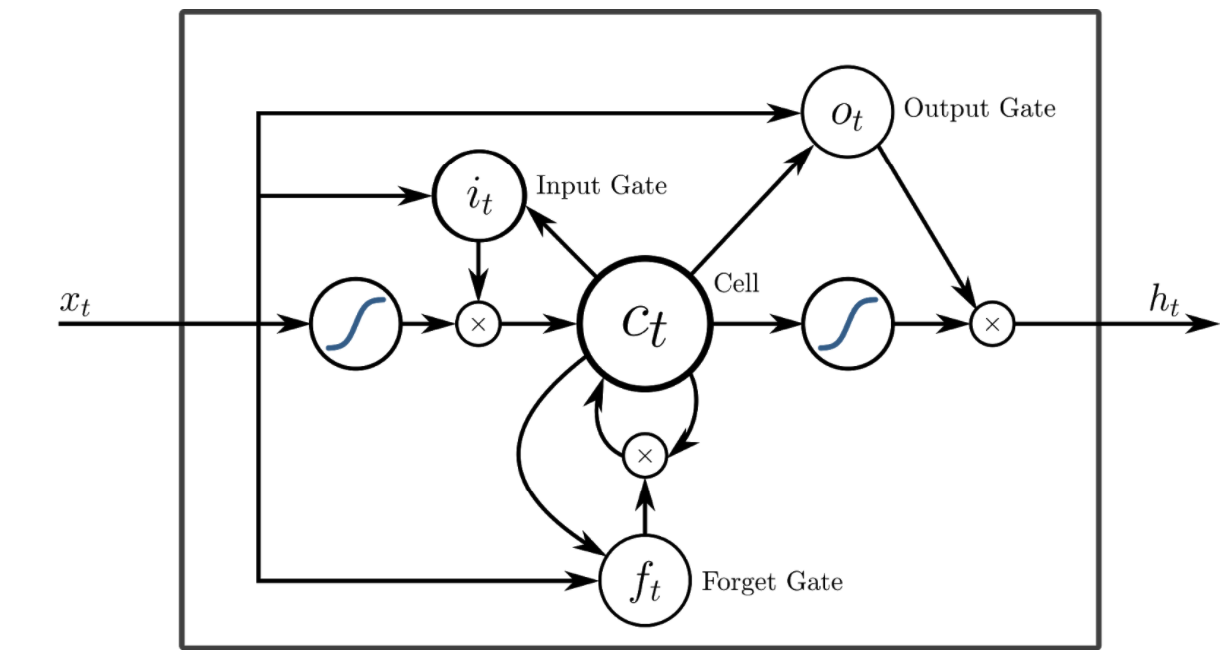
LSTM is a type of recurrent neural network which was developed to overcome the exploding/vanishing gradient problems of standard RNNs (Hochreiter, 1997). LSTMs contain a memory cell that can store information for longer periods of time. This cell has a set of gates used to control when information enters the memory, when it's output, and when it's forgotten, making them effective at capturing the long-distance dependencies in written text
As a result, they have been used as state-of-the-art models in numerous sequence learning tasks, such as time series prediction, but also part of speech-tagging and text classification.
However, one issue with the typical LSTM structure is that it considers all input data to be sequential. In order to to retain the option of including non-sequential features, such as numerical or lexical features, we opted for a hybrid approach which takes two inputs (fig. 2)
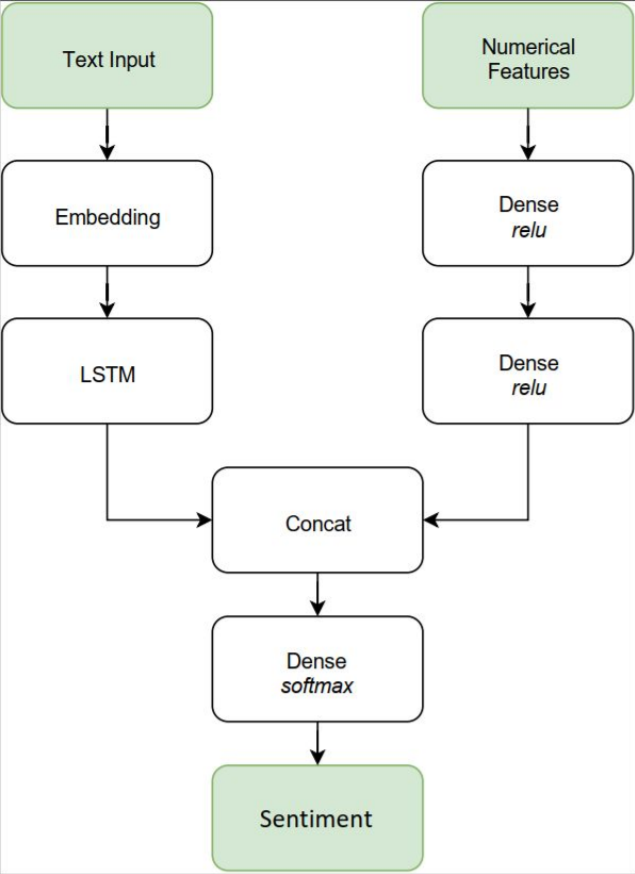
The left-hand side takes the processed text input and uses an embedding matrix to generate word embeddings which are then passed to the LSTM cell. The right-hand side is a simple neural network architecture with a couple of dense layers that deals with the numerical features. After the LSTM adjusts the weights of our sequential data the output is concatenated with the remaining features.
Sentiment Lexicon
The most promising numerical feature we implemented was based on a sentiment lexicon. We mention lexicon-based approaches previously, as we point out that they lag behind machine learning approaches in perfomance by themselves. However, we found lexicon-driven features to be an excellent way to augment our model.
Our features are based on the SentiWords sentiment lexicon (Gatti et. al, 2016), which contains approximately 155.000 words, along with a sentiment score ranging from -1 to 1. These scores were used to create cumulative positive and negative ratings of each comment. Additionally we included the number of both positive and negative words contained in the comment. Because the dataset we had is generally very opinionated, this proved to be a good way to gauge the overall disposition of the text.
Discussion
In this section we will summarize the performance of both approaches we used, as well as discuss some obstacles we encountered in the process of performing Sentiment Analysis. The accuracy of the models generated for each approach can be found in the table below (note: the models that were trained for only one question were evaluated on their performance on that question only).
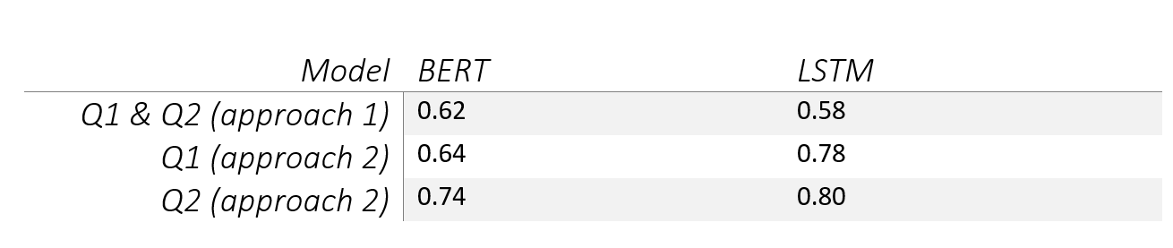
Looking at the accuracy of both architectures, the LSTM performed marginally better on the given dataset. However, while the results were more or less similar, the difference in computation speed between BERT and LSTM were considerable. Even when using the smallest available model at the time, the classification process of the whole dataset using the BERT approach was so computationally expensive it took multiple hours. In contrast, the LSTM can classify the entire dataset in less than 15 minutes.
Despite being easy to set up, a BERT-based approach does not seem like a suitable solution, given its unsatisfactory performance and exorbitant computational costs. Ultimately, we decided to include the LSTM model in our pipeline, given that it achieved comparable results to BERT but was significantly faster with respect to training and classification.
One issue we did not anticipate was related to the dataset itself and can partly explain the mediocre performance of both approaches we used. While open-ended survey answers should be relatively easy to classify, the way the data is split between the two questions complicates the task. One possible improvement could be to filter the data better, considering only longer, less ambiguous sentences for classification, and leaving out very short, contextual comments.
In addition, more training data is always better. However, labeling data with sentiment information is not a trivial task even for humans. Labeling more comments, while tedious, could lead to better results, but it would have also required formulating some more strict guidelines that the annotators can follow. Since the annotation was done by members of the group, investing more time in it meant less focus on the implementation, so it did not represent a priority for us at the time.
References
| [1] | aswani, Ashish & Shazeer, Noam & Parmar, Niki & Uszkoreit, Jakob & Jones, Llion & Gomez, Aidan N. & Kaiser, Lukasz & Polosukhin, Illioa. (2017). Attention is all you need. |
| [2] | Chen, Long-Sheng & Liu, Cheng-Hsiang & Chiu, Hui-Ju, 2011. "A neural network based approach for sentiment classification in the blogosphere," Journal of Informetrics, Elsevier, vol. 5(2), pages 313-322. |
| [3] | Devlin, Jacob & Chang, Ming-Wei & Lee, Kenton & Toutanova, Kristina. (2018). BERT: Pre-training of Deep Bidirectional Transformers for Language Understanding. |
| [4] | E. Cambria, "Affective Computing and Sentiment Analysis," in IEEE Intelligent Systems, vol. 31, no. 2, pp. 102-107, Mar.-Apr. 2016, doi: 10.1109/MIS.2016.31. |
| [5] | Gatti, L., Guerini, M., & Turchi, M. (2016). SentiWords: Deriving a high precision and high coverage lexicon for sentiment analysis. IEEE Transactions on Affective Computing, 7(4), 409-421. |
| [6] | Hochreiter, Sepp & Schmidhuber, Jürgen. (1997). Long Short-term Memory. Neural computation. 9. 1735-80. 10.1162/neco.1997.9.8.1735. |
| [7] | Lan, Z., Chen, M., Goodman, S., Gimpel, K., Sharma, P., & Soricut, R. (2019). Albert: A lite bert for self-supervised learning of language representations. arXiv preprint arXiv:1909.11942. |
| [8] | Liu, Y., Ott, M., Goyal, N., Du, J., Joshi, M., Chen, D., ... & Stoyanov, V. (2019). Roberta: A robustly optimized bert pretraining approach. arXiv preprint arXiv:1907.11692. |
| [9] | Munikar, Manish & Shakya, Sushil & Shrestha, Aakash. (2019). Fine-grained Sentiment Classification using BERT. |
| [10] | R. Liu, Y. Shi, C. Ji and M. Jia, "A Survey of Sentiment Analysis Based on Transfer Learning," in IEEE Access, vol. 7, pp. 85401-85412, 2019, doi: 10.1109/ACCESS.2019.2925059. |
| [11] | Sanh, V., Debut, L., Chaumond, J., & Wolf, T. (2019). DistilBERT, a distilled version of BERT: smaller, faster, cheaper and lighter. ArXiv, abs/1910.01108. |
| [12] | Wang, Jin & Yu, Liang-Chih & Lai, K. & Zhang, Xuejie. (2016). Dimensional Sentiment Analysis Using a Regional CNN-LSTM Model. 225-230. 10.18653/v1/P16-2037. |
| [13] | Yang, Z., Dai, Z., Yang, Y., Carbonell, J., Salakhutdinov, R. R., & Le, Q. V. (2019). Xlnet: Generalized autoregressive pretraining for language understanding. In Advances in neural information processing systems (pp. 5753-5763). |
| [14] | Zhang, L., Zhou, Y., Duan, X., & Chen, R. (2018). A Hierarchical multi-input and output Bi-GRU Model for Sentiment Analysis on Customer Reviews. |