Overview  Data Preparation  Topic Modeling  Sentiment Analysis  Outcome and Reflection 

Topic Modeling

Introduction

As mentioned in the Overview section of this report, our topic analysis pipeline employs a document clustering approach which dynamically-identifies an optimal clustering of vectorized document representations, before passing clustered documents onto later tasks such as Sentiment Analysis. However, it must be admitted that this approach is not the most-common method for achieving the task of topic modeling, and we below provide an overview of the task of topic modeling to contextualize the subsequent deep-dive into our methodology.

Topic modeling is the natural language processing (NLP) task of identifying representative groups of topics in a text dataset. In other words, when provided a set of documents, an effective topic modeling will demonstrate 'what the documents are about.' Given that we implement a topic modeling pipeline for reporting on open employee survey comments, reasonable topics identified by a successful modeling may include topics such as salary, teamwork, etc.

There exist two main approaches to the topic modeling task: statistical topic model approaches and document clustering approaches. We briefly describe the statistical approach before investigating our methods.

Digression: Statistical Topic Modeling Approach

Statistical topic modeling approaches assume generative language models and aim to identify the "latent" or hidden topic correlations between corpus documents via statistical inference. The most commonly employed statistical topic model, which we also explored for our use-case, is Latent Dirichlet Allocation (LDA), originally proposed by Blei et al. (2003) [2]. Figure 1 demonstrates the generative model informing the LDA topic model, where a per-document topic distribution α and per-document word distribution β generate, respectively and in conjunction, the distribution of topics in a document and ultimately a single word w as an outcome of the distribution of words in a latent topic. In other words, by assuming a set of topics each constituted by a distribution of words, documents are interpreted as an outcome of a distribution of topics for a number of words N.

where:

• α is the per-document topic distributions
• β is the per-topic word distribution
• θ is the topic distribution for document m
• z is the topic for the n-th word in document m
• w is the specific word
• N is the number of words in a given document
• M is the number of documents

Figure 1: Plate diagram of LDA model.

Under this model, the words w are the only observable features of documents used to infer the other parameters for a given corpus. There exist various approaches to this statistical inference problem, e.g. Monte Carlo simulation.

We employ an out-of-the-box library for LDA analysis on our dataset. The dataset consists of 17672 documents with 343549 words where 20% are used as test data and 80% as training data. For a comprehensive list of the preprocessing steps employed, please refer to the Data Preparation section of this report.

One challenge with LDA is that the number of topics for a given dataset is a free parameter. This means that one must train the model with an arbitrary number of expected topics k. However, by training on the same dataset for different k values and observing the values of certain inferred parameters, one can make informed guesses as to the most-suitable number of topics. The c_v and UMass coherence scores both provide a quantitative measure of the 'quality' of inferred topics. For both scores, a higher value is preferable, with a c_v score above 0 indicating a good topic modeling. Figure 2 shows the c_v coherence scores for a variety of k values, and word clouds of the inferred topics for the highest value of k = 8 (c_v = 0.37).

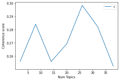
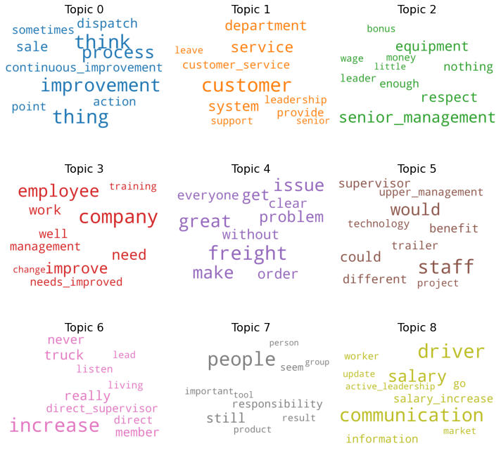
Figure 2: Topic coherence and word clouds for LDA topic modeling.

Metrices	Coherence Score	Number of Topics
c_v (0 < x < 1)	0.37	8
u_mass (-14 < x < 14)	-5.84	8

Table 1 : Coherence measures the distance between words within a topic. The c_v and u_mass metrics are 0.37 and -5.84 for 8 topics respectively.

In sum, the LDA statistical topic model approach yields reasonable results for our dataset, even considering the challenge of determining the free parameter k. In later sections, we describe our alternative approach to the topic analysis task, which leverages pretrained word vectors and document clustering. The Outcome section of this report documents the resulting topics identified under this alternative methodology.

Document Clustering Pipeline

As stated, we employ a document clustering approach given our academic interest in exploring the applications of pretrained word embeddings coupled with traditional cluster analyses. Furthermore, we ignore supervised approaches such as document classification because these are unsuitable for our task given the requirement that the pipeline be able to dynamically-identify new topics potentially unrepresented in a training set.

The document clustering approach requires that we first transform the unstructured comment data into numerical features before performing a cluster analysis on the feature-engineered documents. After feature-engineering we obtain document vectors for which we perform a cluster analysis optimized via hyperparameter grid search, before generating meaningful topic labels useful for report generation. The below image summarizes the topic modeling pipeline as implemented in our codebase.

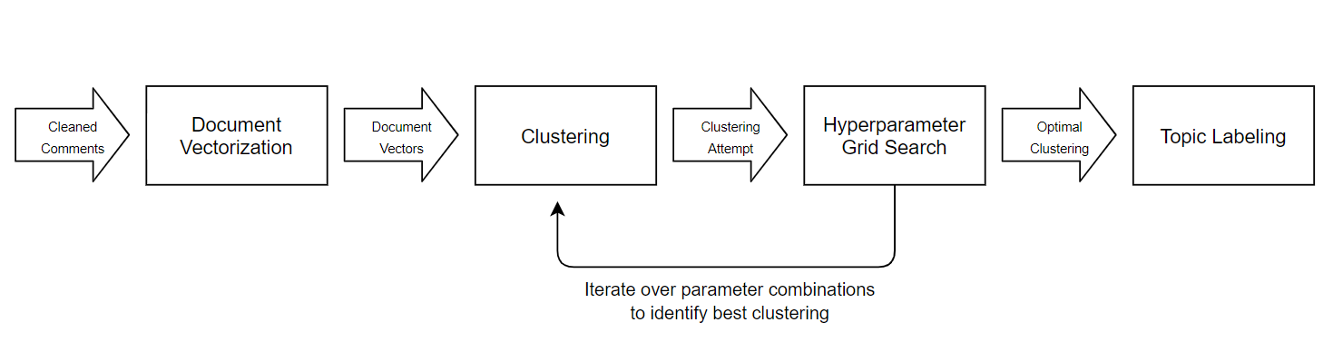Figure 3: Diagram of Topic Modeling Pipeline.

Document Vectorization

While it is a trivial task to obtain word vectors from pretrained neural word embedding models such as word2vec or FastText, it is challenging to devise a methodology for converting these word-level vectors into a normalized document representation which still encodes the semantic information of the document's concatenated tokens.

Many solutions to the problem of document vectorization leverage the demonstrated compositionality of obtained word embeddings, i.e. the behavior that larger blocks of information such as phrases can be represented by the vector manipulation of embedding constituents. [1] Due to this property of trained word embeddings, one can negotiate vector operations such as addition to superficially 'combine' the semantic information encoded in individual tokens into a document representation.

A naïve solution for obtaining a document vector is the simple average of embedding vectors constituting a document. As an initial approach, we employed this method for obtaining document vectors, but the resulting clusterings did not yield optimal results. The figure below demonstrates a sample clustering on FastText vectors averaged to obtain document vectors. Clearly, the clusters are not clearly separable.

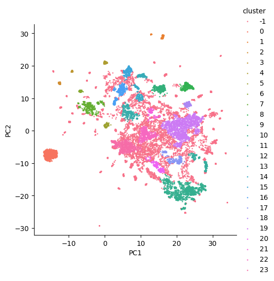Figure 4: Cluster analysis with average word vectors.

It has been shown that weighting embeddings via smoothed term frequency can improve performance on text similarity tasks without the need for additional training data. [3] Because of these findings, we opted to implement additional functionality for computing the smooth-inverse-frequency (SIF) weighted average of word embeddings as a document representation. The SIF weighting equation for a single word is demonstrated below:

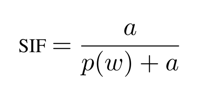
where a denotes an arbitrary normalization constant of approximately 1e-5, and p(w) denotes the word's frequency. Nevertheless, preliminary evaluations showed that this baseline, although effective for text similarity, did not generalize well to the creation of document vectors which performed effectively for document clustering.

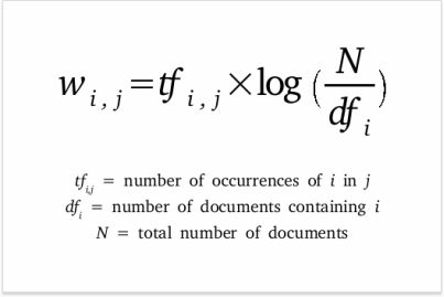
Inspired by research into effective document representations for twitter sentiment analysis, a domain which is somewhat comparable to ours given similarities between twitter texts and our short, focused comments, we opted to integrate into the SIF weighted average the Term-Frequency-Inverse-Document-Frequency (TFIDF) measure as a replacement for the value p(w), as was found to be itself effective as a weighting schema for document vectors [4, 5]. With this modification, the weighting equation for single words in our averaged document vectors becomes

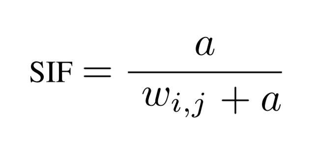
where w for a term i in document j denotes

The resulting weighting scheme produces satisfactory clusterings when qualitatively compared with other approaches. Seen below, a sample clustering with increased separation between identified clusters suggests that the TFIDF weighting scheme captures the most-relevant keywords of each document and effectively weights these terms in order to generate more meaningfully-distinct document vector representations.

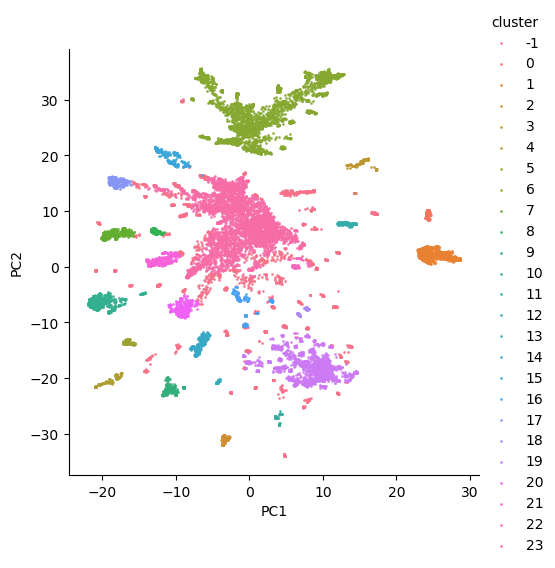Figure 5: Cluster analysis with smooth-inverse-tfidf vectors.

Dimensionality Reduction

Dealing with High Dimensional Datasets

When we work with natural language, we often have to deal with a large amount of data. If such a dataset also contains many different variables, we speak of a so-called high dimensional dataset. For a lot of scientific tasks such high dimensional datasets are a welcome basis, but as Spiderman's uncle might say „with high dimensional datasets comes the great curse of dimensionality". Working with large data sets entails problems, such that it requires a lot of time and space complexity, it often leads to overfitting, not all the features in the given data set might be relevant to our problem and, due to the many dimensions, we are unable to visualize our data set. And finally the curse of dimensionality hits us.

The curse of dimensionality refers to a phenomenon that occurs when working with high dimensional data. With the curse of dimensionality we facing two kinds of problems: one is the data sparsity and the other one is the closeness of the data.

Data Sparsity The volume of the represented space grows quicker than the data and thus becomes sparse. This is a problem if we want to derive some statistical significance from the data

Figure 6: Demonstration of data sparsity. Source

Closeness of the Data In low dimensional spaces, data may seem very close but the higher the dimension the further these data points may seem to be. In other words, distances of objects seem to be different when changing perspectives.

Figure 7: Objects appear differently from different perspectives. Source

In other words: when the number of features or dimensions grow, the amount of data we need to generalize accurately grows exponentially. That makes common data organization strategies become inefficient.

Dimensionality Reduction Techniques

There is a trick that helps us to organize, reduce and visualize such large amounts of data: it’s called dimensionality reduction. Dimensionality reduction is about discovering non-linear and non-local relationships in a given high dimensional data set. By reducing the dimensions we can reduce noise in the data which in turn makes it easier to apply simple learning algorithms. In our project, we are applying the following two dimensionality reduction techniques:

• Principle Component Analysis (PCA)
  PCA is the most tried linear dimensionality reduction technique. It transforms existing variables into a new set of variables, which are a linear combination of the original variables and finally converts the correlations among all of the features into a 2D-Graph. What we can see after applying PCA is that features that are highly correlated cluster together whereas the differences along the first principal component axis are more important than the differences along the second principal component.
  
  
• Uniform - Manifold Approximation and Projection (UMAP)
  UMAP is a non-linear dimensionality reduction technique with a solid mathematical background. Its algorithm balances between emphasizing local versus global structure. After first modeling a blurry topological structure of the high dimensional set it is searching for a low dimensional projection that is closest to it.
  

Results

In our pipeline we are applying both dimensionality reduction techniques: first PCA and following UMAP. Doing so we expected to get an improved computation time and to obtain a less noisy dataset. In Figures 10 and 11, you can observe the apparent difference in dataset topography when reducing dimensions with UMAP alone and with PCA and UMAP combined.

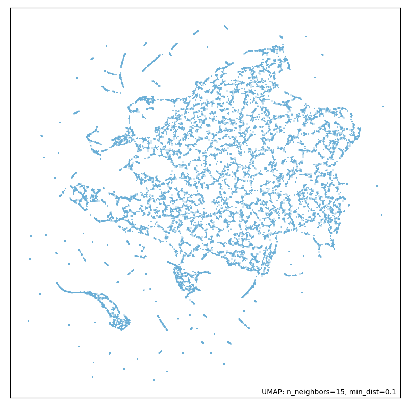
Figure 8: Running dimensionality reduction only with UMAP (without PCA).

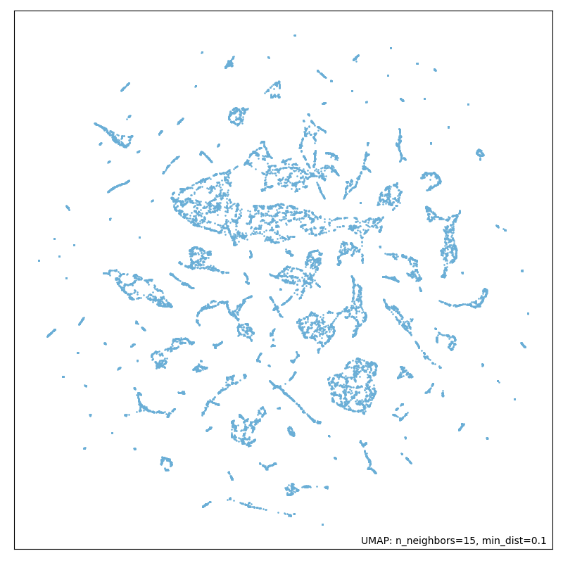
Figure 9: Running dimensionality reduction with UMAP and PCA.

Our expectation in obtaining a less noisy dataset by applying both algorithms has been fulfilled. We can see the difference by looking at the first picture which is a plot of the dataset after only applying UMAP, in contrast to the second picture where we can see a plot of the dataset after applying PCA and UMAP in combination. The output is more precise and structured. These results supported our approach.

Clustering

Introduction

Clustering is a method where similar or similar properties of data points are group together Given a set of data points, we can just use a clustering algorithm to search for patterns in the given scenario, finding similarities within the data and group them together.

Clustering Algorithms can be divided into Four types :

• Flat and Centroid based
• Flat and Density based
• Hierarchical and Centroid based
• Hierarchical and Density based

Figure 10: Overview of cluster algorithms.

The above picture shows the overall idea of clustering types. Flat and Centroid based alogorithms such as K-means clustering enforce prior assumptions on the shape of the clusters. It works very well on defined shapes of clusters such as circular, rectangular, etc also works best when we have small amount, low dimensional data. But when we have higher dimensional data and also no prior knowledge of shapes of cluster, then k-means performs very poorly, and in such case we prefer to use Flat and Density based such as DBSCAN clustering which is short form of Density Based Spatial Clustering. DBSCAN works very best on for clusters of different shapes, variable densities, variable sizes and datasets have noises in data. It's very difficult to judge the number of clusters in a dataset, what can be the best parameter settings for number of clusters? Hierarchical based algorithms solve this problem, Hierarchical and Centroid based algorithm such as Agglomertive Hierarchical clustering which splits all the data points and make a dendogram and then clusters are fromed from the branches. Since we are dealing with very high dimensional data with lots of noise, we chose to use HDBSCAN which is mixture of DBSCAN and Hierarchical based algorithm.

HDBSCAN

HDBSCAN works on DBSCAN, DBSCAN has two parameters that are : epsilon and min-points. epsilon is radius of a circle, which enclose data points, and if data points inside 'eps'(epsilon) radius are above K(min-points) then the circle considered as Dense Circle. In HDBSCAN, the parameter min-points are passed and fixed for DBSCAN, and different epsilon radius circle are drawn, and then HDBSCAN algorithm looks for the smaller eps value which accomodate min-points. And that eps value considered as dense. The circles get merged using Probability density function and using distance metrics Mutual Rechability Distance components get connected forming minimum spanning tree. Next step in HDBSCAN is to convert MST into the hierarchy of connected components, using sorting of edges of MST which is also converted in Dendogram. HDBSCAN takes a parameter minimum cluster size, to eradicate clusters that has lower data points than minimum cluster size. Afterwards, HDBSCAN takes another parameter which acts as threshold which cut out the condensed dendogram, the maximum points in the hierarchy considered as clusters. For more info see here Cluster Extraction

This is how HDBSCAN algorithm performs, in project we used the package from Scikit learn. The most important parameters which we already discussed above are min_cluster_size, metric and min_samples.

Topic Labeling

The aim of this pipeline step is to find suitable labels for each previously identified cluster. The topic labeling is performed on the pre-processed data. Importantly, the comments no longer contain stop-words and the words are lemmatized (e.g. talk instead of talks or talked ). Generally, finding an appropriate label for a document is a difficult task for computational automation, because no one unique solution exists. Typically, a range of possible labels are appropriate for the document and humans prefer abstract labels which will likely consist of words not found in the text of the document. For this reason the approach presented here focuses on easy methods on the basis of words occurring in the comments, because this makes the process faster and less resource-intense.

As a basis for labeling and a brief characterisation of the cluster a set of keywords is determined for each cluster. This is done using either the unaltered word frequency or TFIDF. TFIDF takes into account besides the frequency of the word in question itself also the rarity of this word across different comments in the cluster. This technique is typically employed to counteract the effect of very frequent words which have a high frequency across all inspected documents. In this case, as common stop-words are already removed in the data preparation, word frequency and TFIDF perform similarly.

The label is then chosen by projecting the keywords back into embedding space and selecting the mean as a label for the cluster. Alternatively, a simpler method takes the five most common keywords in the cluster and uses this list as a label for the cluster. The advantage of the mean projection is that a single-word label instead of a list of words is better aligned with how a person might choose a cluster label.

For additional insight into the content of the identified clusters we attempted to select a few representative comments for each cluster. We implemented two different approaches for this task: a statistical approach and an embedding-focused approach. The statistical approach utilizes the frequency distribution of all words in the cluster. This frequency distribution is calculated and then normalized by dividing it through the frequency of the most frequent word. Each comment is assigned a weight which is the sum of all normalized frequencies of the words in the comment. The comments with the highest weights are taken as most representative of the cluster. This approach as described above introduces a bias toward longer comments, because the weight is not normalized by the number of words in the comment. In the embedding-focused approach we calculate the centroid embedding of all embeddings representing the comments in the cluster by taking the mean of each dimension. This centroid embedding then forms a reference point and we determine the cosine distance of each comment embedding to the centroid embedding. The comments with the smallest cosine distance are taken as representative of the cluster. The quality of representative comments selected with this approach depends on the structure of the underlying cluster. If a few comments in the cluster are very different from the rest these “outliers” will skew the resulting mean.

In conclusion, the simple methods presented here can provide some insights into the contents of the clusters and are applicable to all contents, but do not reach the quality of human-like annotation. Additionally, the resulting labels highly depend on the quality of the underlying data and clustering especially the degree to which clusters form coherent groups and are separated from each other.

Optimization: Finding the Best Parameters with Grid Search

The algorithm

In general, a grid search is nothing else than successively trying out different function input parameter configurations, then measuring the performance for each configuration with a predefined score. The ultimate goal is to maximize this score to get the best possible setting for the underlying problem. The name grid search comes from the visualization in which each of the configurations can be seen as a node of a grid in a high dimensional vector space (e.g., a cube in a 3-dimensional parameter space).

Our approach

The general definition of grid search is scanning the data to configure the optimal parameters for a model. In our topic model approach, this means something slightly different, namely finding the best parameters for the different components of the topic modeling pipeline (e.g., normalization, dimensionality reduction, clustering).

To implement a smooth and dynamic grid search process, we had to adjust our underlying pipeline architecture in a very standardized but also flexible way. To this end, we gave every component function a fixed structure, which requires as input the data, the name of the used algorithm, and the parameter configuration. With this structure, it is easy to switch or drop out specific components, or for our case, it was straightforward to call the functions in sequence for the grid search.
We implemented a pipeline variable (Figure 11) for the actual process, which is basically a python dictionary that contains all information about the grid search components. So it is built with all different functions and a bunch of input parameters, which then make the grid:


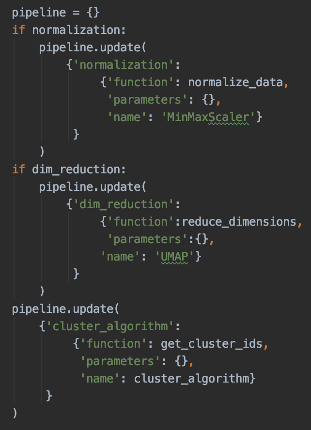
Figure 11: Adding normalization, dimensionality reduction and clustering algorithm to the pipeline.

The actual grid search was implemented in a highly dynamic way fitting the pipeline structure. This allows a component to be integrated into the pipeline by merely adding it to the pipeline variable with the required information. This process is possible due to providing the python function, for example, for the clustering algorithm as a kind of object variable in order to enable simple iterating through these successive components. Surely, they have to be designed in a way that the previous functions' output suits the input of the upcoming one.
Our grid search aims to optimize the so-called silhouette score, which measures how close the points of one cluster are compared to the distance between the different clusters. We found the best parameter configuration by optimizing this score, which we then set as default for our topic modeling pipeline. Additionally, for a cross-check, we also took the number of outliers into account.

Logging

Running a grid search without logging the information you get during the process is pointless. Therefore, we paired each configuration with the associated scores. The pairs were sent to our Mongo database to ensure saving even if the grid search stopped prematurely. Simultaneously, this step enabled access from remote working stations. With the python library pymongo , a connection to the database was set up by creating a python dictionary with all critical information and storing it in a grid search collection. The library automatically converts the python dictionary to a MongoDB object. Additionally, we implemented some sort of wrapper for smoother handling of the information in the database. This wrapper allowed us to write, delete, and search for database objects so that the best configurations' information remains accessible at any point.

Evaluation: Analyzing the Outcome of the Grid Search

Our Approach

In addition to figuring out the best configurations from the grid search descriptively, we analyzed the grid search logs by means of a multiple regression analysis to assess how much the different parameters contribute to the silhouette score. The six predictors entered in the regression were the grid search parameters defining the functioning of the UMAP dimensionality reduction algorithm and the hdbscan clustering algorithm. Their metric (Canberra/Cosine/Euclidean and Canberra/Euclidean, respectively) was entered as a predictor for both algorithms. Additionally, for UMAP the number of neighbors and the spread were taken into account, and for hdbscan, the minimum cluster size and the minimum number of samples. All predictors were treated as categorical data because only a few distinct values of the usually continuous parameters could be entered into the grid search due to the limited computational power available.
As the grid search was run twice, once for the pipeline based on Fasttext embeddings and once based on BERT embeddings, two analyses were conducted and are presented separately. Our goal with both analyses was to find a straightforward solution employing only predictors that contribute substantially to the explained variance while accounting for as much variance as possible. The dependent variable is the silhouette score; the outliers were not included as a dependent variable. However, to reduce noise in the data, we excluded results with more than 10% outliers from the analyses. Additionally, results presenting more than 375 clusters were also excluded, as such a high number of clusters seemed unreasonable given our input data.

Results with Fasttext embeddings

We identified a linear model employing the ordinary least squares (OLS) technique with four predictors and no interactions, that accounts for 67.24% of the variance in our data (F(5, 624) = 259.9, p < 0.001, R² = 0.6755, Adjusted R² = 0.6729). According to these results, the best parameter combination is the Cosine metric, an increased number of neighbors, and larger cluster size for UMAP, as well as a smaller number of samples for hdbscan (Table 2).

	Estimate	Std.Error	t-value
Intercept	-0.19768	0.00463	-42.731   ***
UMAP: metric cosine	0.08805	0.00314	28.080   ***
UMAP: metric euclidean	0.02838	0.00314	9.050   ***
UMAP: number of neighbors	0.00105	0.00010	10.267   ***
hdbscan: min cluster size	0.00068	0.00004	17.929   ***
hdbscan: min number of samples	-0.00102	0.00033	-3.085   **

Table 2: Results of the multiple regression analysis of the grid search logs based on fasttext embeddings.
Significance codes: '***' 0.001    '**' 0.01    '*' 0.05
R² = 0.6755, Adjusted R² = 0.6729, AIC = -2532.875

Results with BERT embeddings

The results look different for the grid search logs generated using the pipeline with BERT embeddings. As the precondition of homoscedasticity was not satisfied, we employed a regression with the generalized least squares technique (GLS). The best model here comprises three predictors and one interaction. The implied advice here is to use the Euclidean metric for both algorithms and increase the minimum cluster size for the hdbscan algorithm (Table 3).

	Value	Std.Error	t-value
Intercept	-0.10262	0.01211	-8.474   ***
UMAP: metric cosine	0.00123	0.01415	0.087    n.s.
UMAP: metric euclidean	0.04785	0.014146	3.383   ***
hdbscan: metric euclidean	0.05686	0.01412	4.026   ***
hdbscan: min cluster size	0.00163	0.00012	14.117   ***
Interaction: UMAP metric cosine x hdbscan metric euclidean	-0.02125	0.01999	-1.063    n.s.
Interaction: UMAP metric euclidean x hdbscan metric euclidean	0.16369	0.01997	8.195   ***

Table 3: Results of the multiple regression analysis of the grid search logs based on BERT embeddings.
Significance codes: '***' 0.001    '**' 0.01    '*' 0.05
AIC = -1186.359 BIC = -1147.218 logLik = 601.1795

Conclusion

Following the results of the regressions, straightforward advice on optimizing the pipeline can be given; however, this advice's limitations should be considered in the process. Most importantly, since a reasonable number of clusters is limited from a theoretical point of view, the results of a correspondingly limited grid search would likely provide more accurate insights. Furthermore, the regression models do not fit the data perfectly, thereby possibly limiting the validity and generalizability of the results. The noise in the original data can at least partly explain the reduced fit. To sum, the regression helps to shed light on the parameters that most decisively contribute to the score; nevertheless they should not lead to the omission of a close inspection of the configurations.

Discussion

Our topic modeling approach is only one of several possible approaches, and was primarily chosen given our interest in utilizing new, state-of-the-art technologies such as pretrained neural word embeddings. Due to the unsupervised nature of our approach and the data's features (short comments, spelling and grammar errors), our approach remained difficult to optimize and is open to several areas for improvement.

The disadvantage of using pretrained language embeddings is that there currently exists little literature regarding the behaviour of these models in novel use-cases. For example, it is unclear how the assumptions of the document vectorization methodology we employ can extend to both the FastText and BERT vectors. Given that our approach leverages the compositionality of static word vectors and is designed to compensate for a lack of contextual information in these constituents, it may be that the weighted-TFIDF schema is inappropriate for contextual BERT vectors, and rather introduces unnecessary noise which problematizes the analysis when using these pretrained vectors. Further investigation into the effects of the TFIDF-weighting schema on BERT vectors would help to elucidate this concern.

A further difficulty is the large number of tunable parameters producing demanding computation times when running the grid search. As demonstrated through regression analysis, many of these parameter ranges can be trimmed. Additionally, counter to our intentions the pipeline may produce different results even when configured with consistent parameters. This behaviour is a result of the uncontrollable stochasticity inherent to some off-the-shelf machine learning methods we employ. For example, the HDBSCAN algorithm is not entirely deterministic, rendering efforts to control for randomness elsewhere in the pipeline effectively moot, and the results of the grid search questionable under these circumstances.

Back to Top

References

[1]	Mikolov, Tomas & Corrado, G.s & Chen, Kai & Dean, Jeffrey. (2013). Efficient Estimation of Word Representations in Vector Space. 1-12.
[2]	Blei, David & Ng, Andrew & Jordan, Michael. (2001). Latent Dirichlet Allocation. The Journal of Machine Learning Research. 3. 601-608.
[3]	P. Bojanowski, E. Grave, A. Joulin, T. Mikolov. (2016) Enriching Word Vectors with Subword Information.
[4]	Arora, S., Liang, Y., & Ma, T. (2016). A simple but tough-to-beat baseline for sentence embeddings. Paper presented at 5th International Conference on Learning Representations.
[5]	Edilson Anselmo Correa Junior, Vanessa Marinho, and Leandro Santos. (2017). NILC-USP at SemEval-2017 Task 4: A Multi-view Ensemble for Twitter Sentiment Analysis. In Proceedings of the 11th International Workshop on Semantic Evaluation. Vancouver, Canada, SemEval ’17, pages 610–614.
[6]	Zhao, Jiang & Lan, Man & Tian, Jun. (2015). ECNU: Using Traditional Similarity Measurements and Word Embedding for Semantic Textual Similarity Estimation.
[7]	M. Röder, A. Both, A. Hinneburg, 2015. Exploring the Space of Topic Coherence Measures
[8]	J. K. Pritchard, M. Stephens and P. Donnelly, 2000. Inference of Population Structure Using Multilocus Genotype Data
[9]	S. Hochreiter, P. Schmidhuber, 1997. Long short-term memory.